Programs and Probability
By Brian Hayes
Computer programs must cope with chance and uncertainty, just as people do. One solution is to build probabilistic reasoning into the programming language.
Computer programs must cope with chance and uncertainty, just as people do. One solution is to build probabilistic reasoning into the programming language.

DOI: 10.1511/2015.116.326
Randomness and probability are deeply rooted in modern habits of thought. We meet probabilities in the daily weather forecast and measures of uncertainty in opinion polls; statistical inference is central to all the sciences. Then there’s the ineluctable randomness of quantum physics. We live in the Age of Stochasticity, says David Mumford, a mathematician at Brown University.
Ours is also an age dominated by deterministic machines—namely, digital computers—whose logic and arithmetic leave nothing to chance. In digital circuitry strict causality is the rule: Given the same initial state and the same inputs, the machine will always produce the same outputs. As Einstein might have said, computers don’t play dice.
But in fact they do! Probabilistic algorithms, which make random choices at various points in their execution, have long been essential tools in simulation, optimization, cryptography, number theory, and statistics. How is randomness smuggled into a deterministic device? Although computers cannot create randomness de novo, they can take a smidgen of disorder from an external source and amplify it to produce copious streams of pseudorandom numbers. As the name suggests, these numbers are not truly random, but they work well enough to fool most probabilistic algorithms. (In other words, computers not only play dice, they also cheat.)
A recent innovation weaves randomness even more deeply into the fabric of computer programming. The idea is to create a probabilistic programming language (often abbreviated PPL and sometimes pronounced “people”). In a language of this kind, random variables and probability distributions are first-class citizens, with the same rights and privileges as other data types. Furthermore, statistical inference—the essential step in teasing meaning out of data—is a basic, built-in operation.
Most of the probabilistic languages are still experimental, and it’s unclear whether they will be widely adopted and prove effective in handling large-scale problems. But they have already provided an intriguing new medium for expressing probabilistic ideas and algorithms.
Suppose you throw three standard dice, colored red, green, and blue for ease of identification. What are the chances of scoring a 9? No less a luminary than Galileo Galilei took up this question 400 years ago—and got the right answer! His method was enumeration, or counting all the cases. Each die can land in six ways, so the number of combinations is 63, or 216. If the dice are fair, all these outcomes are equally likely. Go through the table of 216 combinations and check off those with a sum of 9. You’ll find there are 25 of them, giving a probability of 25/216, or 11.6 percent.
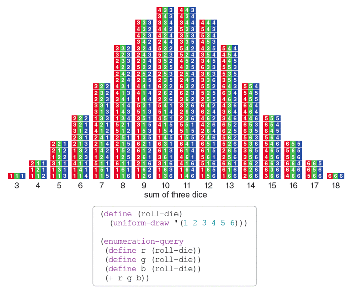
Illustration by Brian Hayes.
Another way to answer the same question is simply to run the experiment: Roll the dice a few million times and see what happens. This sampling procedure is easier with computer-simulated dice than with real ones (an option unavailable to Galileo). In 216 million simulated rolls I got 24,998,922 scores of 9, for a probability within 0.01 percent of the true value.
Enumeration is often taken as the gold standard for probability calculations. It has the admirable virtue of exactness; it is also deterministic and repeatable, whereas sampling gives only approximate answers that may be different every time. But sampling also has its defenders. They argue that randomized sampling offers a closer connection to the way nature actually works; after all, we never see the idealized, exact probabilities in any finite experiment.
In the end, these philosophical quibbles are usually swept aside by practical constraints: Enumerating all possible outcomes is not always feasible. You can do it with a handful of dice, but you can’t list all possible sequences of English words or all possible arrays of pixels in an image. When it comes to exploring these huge search spaces, sampling is the only choice.
The size of the solution space is not the only challenge in solving probability problems; another factor is the complexity of the questions being asked. You may need to estimate joint probabilities (how often do x and y occur together?) or conditional probabilities (how likely is x, given that y is observed?). The most interesting queries are often matters of inference, where the aim is to reason “backwards” from observed effects to unknown causes. In medical diagnosis, for example, the physician records a set of symptoms and must identify the underlying disease. The conclusion depends not only on the probability that a disease will give rise to the observed symptoms but also on the probability of the disease itself in the population. (The formal statement of this principle is known as Bayes’ rule. It’s also implicit in an old saying among diagnosticians: Uncommon presentations of common diseases are more common than common presentations of uncommon diseases.)
The idea of solving probability problems by running computer experiments had its genesis at the Los Alamos laboratory soon after World War II. The mathematician Stanislaw Ulam was playing solitaire while recuperating from an illness and tried to work out the probability that a random deal of the cards would yield a winning position.
After spending a lot of time trying to estimate [the probability] by pure combinatorial calculations, I wondered whether a more practical method than “abstract thinking” might not be to lay it out say one hundred times and simply observe and count the number of successful plays. This was already possible to envisage with the beginning of the new era of fast computers . . .
Ulam’s technique was named the Monte Carlo method, after the famous randomizing devices in that Mediterranean capital. In 1948 the scheme was put to work on a graver task than solving solitaire. A program running on the ENIAC, the early vacuum tube computer, calculated the probability that a neutron moving through a cylinder of uranium or plutonium would be absorbed by a fissionable nucleus before wandering away. (I don’t know if Ulam ever got back to the solitaire problem.)
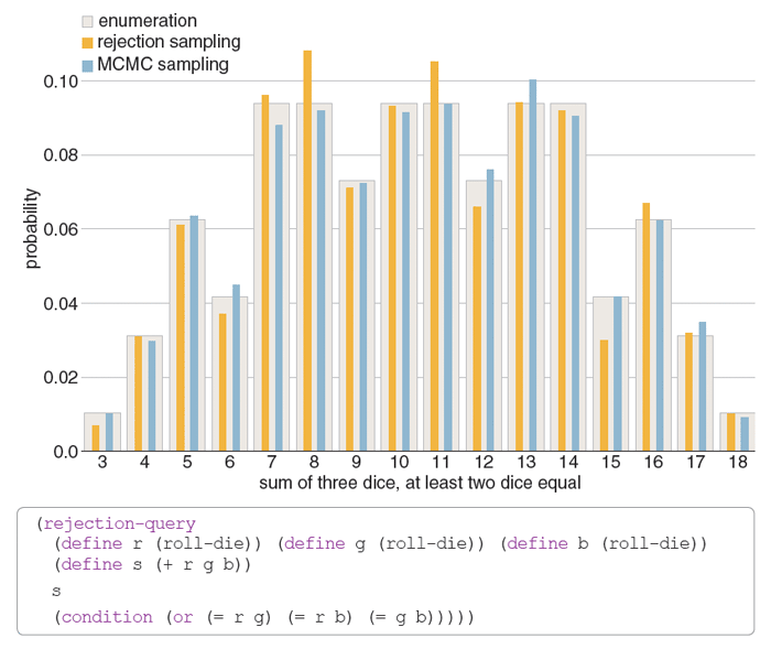
Illustration by Brian Hayes.
The most basic algorithm for sampling is straightforward: Just make repeated trials and tally the results. Where the process gets dicey (so to speak) is with conditional probabilities. Suppose you want to know the probability of rolling a 14 with three dice, on the condition that at least two of the dice display the same number. The simplest approach to such a problem is called rejection sampling. The program simulates many rolls of the dice and discards cases in which the three dice are all different. This procedure is clearly correct; it follows directly from the definition of conditional probability. For the dice problem it works fine, but it becomes woefully inefficient for studying rare phenomena. The program spends most of its time generating events that it immediately throws away. Think of trying to stumble on meaningful English sentences by assembling random sequences of words.
Ideally, we would like to generate only “successes”—states that satisfy the imposed condition—without wasting time on the failures. That goal is not always attainable, but a family of techniques known as Markov chain Monte Carlo (MCMC) can often get much closer than rejection sampling. The basic idea is to construct a random walk that visits each state in proportion to its probability in the observed distribution.
Let’s take a walk through some states of the two-or-more-equal dice game. Assume a roll of the dice comes up red = 2, green = 2, blue = 3, which for brevity we can denote 223. This combination satisfies the two-or-more-equal condition, so we write it down as the initial state of the system. Now, instead of picking up all three dice and throwing them again, choose one die at random and roll that one alone, leaving the others undisturbed. If the result is a state that satisfies the condition, note it down as the next state. If not, return to the previous state and write that down as the second state as well. Continue by choosing another die at random and repeat the procedure. A sequence of states might run 223, 323, 323, 343, 443, 444 . . .
This “chain” of states eventually reaches all combinations that meet the two-or-more-equal criterion. In the long run, moreover, the states in the random walk have the same probability distribution as the one produced by rejection sampling. In subtler ways, however, the MCMC sequence is not quite random. Nearby elements are closely correlated: 223 can make an immediate transition to 233 but not to 556. The remedy is to collect only every nth state, with a value of n large enough to let the correlations fade away. This policy imposes an n-fold penalty in efficiency, but in many cases MCMC still beats rejection sampling.
Monte Carlo simulations and other probabilistic models can be written in any programming language that offers access to a pseudorandom number generator. What a PPL offers is an environment where probabilistic concepts can be expressed naturally and concisely, and where procedures for computing with probabilities are built into the infrastructure of the language. Variables can represent not just ordinary numbers but entire probability distributions. There are tools for building such distributions, for combining them, for imposing constraints on them, and for making inquiries about their content.
A PPL called Church illustrates these ideas. Church was created by Noah D. Goodman, Vikash K. Mansinghka, Daniel M. Roy, Keith Bonawitz, and Joshua B. Tenenbaum when they were all at MIT. Goodman and Tenenbaum’s online book, Probabilistic Models of Cognition ( https://probmods.org), provides an engrossing introduction to Church and to probabilistic programming in general. Readers can modify and run programs directly in the book’s Web interface.
Church is named for Alonzo Church, an early 20th–century logician who developed a model of computation called the lambda calculus. The Church language is built atop Scheme, a dialect of the Lisp programming language that has deep roots in the lambda calculus. Like other variants of Lisp, Church surrounds all expressions with parentheses and adopts a “prefix” notation, writing
(+ 1 2)
instead of
1 + 2
.
Here is the Church procedure for rolling a single die:
(define (roll-die)


  (uniform-draw '(1 2 3 4 5 6)))
When this function is executed, it returns a single number chosen uniformly at random from the list shown. In the larger context of a probabilistic query, however, the result of the
roll-die
procedure can represent a distribution over all the numbers in the list.
The query expression below has three parts: first a list of
define
statements, creating a model of a probabilistic process; second the expression that will become the subject of the query (in this case simply the variable
g); and finally a condition imposed on the outcome:
(enumeration-query


  (define r (roll-die))


  (define g (roll-die))


  (define b (roll-die))


  (define score (+ r g b))


  g


  (condition (> score 13)))
Again we are rolling three simulated dice, designated r, g, and b. The query computes the probability distribution of g subject to the condition that the sum of r, g, and b is greater than 13. The result of running the query is a list giving the possible values of g (2, 3, 4, 5, 6) and their probabilities (ranging from 0.029 to 0.429).
The keyword
enumeration-query
in this program signals that it counts all cases and returns exact results. Substituting the keyword
rejection-query
produces what you would expect: a sampling from the same distribution, performed by discarding cases that fail to satisfy the greater-than-13 condition. A third option is the keyword
mh-query, which invokes a Markov chain Monte Carlo algorithm. (The initials
mh
stand for Metropolis-Hastings; Nicholas Metropolis was a member of the early Monte Carlo community at Los Alamos and W. Keith Hastings is a Canadian statistician.)
The query expressions of Church specify what is to be computed but not how; all the algorithmic magic happens behind the curtains. That’s part of the point of a PPL—to allow the programmer to work at a higher level of abstraction, without being distracted by details of counting cases or collecting samples. Those details still have to be attended to, but the necessary code is written by the implementer of the language rather than the user of it.
Embedding such technology inside a programming language requires algorithms general enough that they work in a variety of problem domains, from playing dice to following neutrons to recognizing faces in images. MCMC simulations often exploit specific features of the problem definition, but a PPL must somehow construct a random walk through the solution space without knowing anything about the nature of the individual states. The strategy adopted in Church is to regard all possible execution paths of the program itself as the elements of the solution space. Each random choice in the program establishes a new branch point in the network of execution paths. The Church MCMC algorithm works by altering one of those choices and checking to see if the new output still satisfies any conditions imposed on the model.
The generic MCMC algorithm is not quite foolproof. Consider another variation on the dice game with a slightly different condition: not (> score 13) but (= score 13). That is, we want to find the distribution of values of the green die when the sum of the three dice is exactly 13. The Church program for this task works fine with an enumeration query or a rejection query, but the MCMC program fails. The reason is that the algorithm always proposes to alter the value of a single die, an action that cannot leave the sum of the three dice unchanged; thus none of the proposals are ever accepted. There are work-arounds for this problem, such as defining a “noisy equal” operator that occasionally judges two numbers to be equal even when they’re not. But the need to understand the cause of the failure and take steps to correct it suggests we have not yet reached the stage where we can blithely hand off probabilistic models to an automated solver.
PPLs are not the only approach to computing with probabilities. The main alternatives are graphical models, in which networks of nodes are connected by lines called edges. Each node represents a random variable along with its probability distribution; an edge runs between two nodes if one variable depends on the other. For example, a network for a model of three dice might look like this:
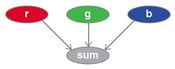
Information flows from each of the dice to the sum, but not between the dice because they are independent.
Advocates of PPLs suggest at least two reasons for favoring a linguistic over a graphical representation. First, certain concepts are easier to encode in a language than in a diagram; an important example is recursion, where a program invokes itself. Second, over the entire history of digital computers, programming languages have proved to be the most versatile and expressive means of describing computations.
Almost 20 years ago Daphne Koller of Stanford University, with David McAllester and Avi Pfeffer, examined the prospects for a probabilistic programming language and showed that programs could be well behaved, running with acceptable efficiency and terminating reliably with correct answers. A few years later Pfeffer designed and implemented a working probabilistic language called IBAL, then later created another named Figaro.
The movement toward PPLs has gathered momentum in the past five years or so. Interest was fortified in 2013 when the U.S. Defense Advanced Research Projects Agency announced a four-year project funding work on Probabilistic Programming for Advancing Machine Learning. At least a dozen new projects have sprouted up. Here are thumbnail sketches of three of them.
WebPPL was created by Noah Goodman (a member of the Church collaboration) and Andreas Stuhlmüller, both now of Stanford University. Like the Web version of Church, it is a language anyone can play with in a browser window, but its roots in Web technology are even deeper: The base language is JavaScript, which every modern browser has built in. An online tutorial, The Design and Implementation of Probabilistic Programming Languages (http://dippl.org), introduces the language.
Stan—which is named for Stanislaw Ulam—comes from the world of statistics. The developers are Bob Carpenter, Andrew Gelman, and a large group of collaborators at Columbia University. Unlike many other PPLs, Stan is not just a research study or a pedagogical exercise but an attempt to build a useful and practical software system. The project’s website (http://mc-stan.org) lists two dozen papers reporting on uses of the language in biology, medicine, linguistics, and other fields.
Meanwhile, some members of the Church group at MIT have moved on to a newer language called Venture, which aims to be more robust and provide a broader selection of inference algorithms, as well as facilities allowing the programmer to specify new inference strategies.
The computing community has a long tradition of augmenting programming languages with higher-level tools, absorbing into the language tasks that would otherwise be the responsibility of the programmer. For example, doing arithmetic with matrices involves writing fiddly routines to comb through the rows and columns. In programming languages that come pre-equipped with those algorithms, multiplying matrices is just a matter of typing A * B. Perhaps multiplying probability distributions will someday be just as routine.
However, PPLs add much more than a new data type. Algorithms for probabilistic inference are more complex than most built-in language facilities, and it’s not clear that they can be made to run efficiently and correctly over a broad range of inputs without manual intervention. One precedent for building such intricate machinery into a language is Prolog, a “logic language” that caused much excitement circa 1980. The Prolog programmer does not specify algorithms but states facts and rules of inference; the language system then applies a built-in mechanism called resolution to deduce consequences of the input. Prolog has not disappeared, but neither has it moved into the mainstream of computing. It’s too soon to tell whether probabilistic programming will become a utility everyone takes for granted, like matrix multiplication, or will remain a niche interest, like logic programming.
Some of the algorithms embedded in PPLs may also be embedded in people. Probabilistic reasoning is part of how we make sense of the world: We predict what will probably happen next and we assign probable causes to what we observe. Most of this mental activity lies somewhere below the level of consciousness, and we don’t necessarily know how we do it. Getting a clearer picture of these cognitive mechanisms was one of the original motivations for studying PPLs. Ironically, though, when we write PPL programs to do probabilistic inference, most of us won’t know how the programs do it either.
©2015 Brian Hayes
Click "American Scientist" to access home page

American Scientist Comments and Discussion
To discuss our articles or comment on them, please share them and tag American Scientist on social media platforms. Here are links to our profiles on Twitter, Facebook, and LinkedIn.
If we re-share your post, we will moderate comments/discussion following our comments policy.