The Fatigue Conundrum
By Ashley Nunes, Philippe Cabon
Whether it’s mild sleepiness or mind-numbing exhaustion, the challenge of fatigue on the job can be complex, dangerous, and surprisingly difficult to manage.
Whether it’s mild sleepiness or mind-numbing exhaustion, the challenge of fatigue on the job can be complex, dangerous, and surprisingly difficult to manage.

DOI: 10.1511/2015.114.218
In 2010, an Air India jet attempting to land in Mangalore, India, overshot the runway and plunged off a cliff, killing 158 people. The ensuing investigation found that the pilot, who was recorded snoring loudly in the cockpit, had committed several critical errors of judgment during the flight, including neglecting the urging of his copilot to abort the landing.

Stringer/Xinhua Press/Corbis
Other failed landings have had less tragic outcomes, such as the American International Airways Flight 808 in 1993 at US Naval Air Station Guantanamo Bay, Cuba. In accordance with standard procedures, the pilot had planned to approach the runway from over the sea and then carry out a late right turn toward the runway so as to avoid entry into Cuban airspace, which began a mere three-quarters of a mile west of the touchdown area. However, the crew, who had been awake for over 19 hours continuously, overbanked the aircraft, causing it to stall and crash. The impact, together with a resulting fire, destroyed the multimillion-dollar aircraft, and the three-member crew suffered serious (although fortunately nonfatal) injuries. As with the Air India crash, an investigation by the National Transportation Safety Board (NTSB) attributed the impaired judgment and flying abilities of the flight crew to the debilitating effects of fatigue.
Since the crash of Flight 808 in 1993, the NTSB and its international counterparts have investigated thousands of transportation accidents, sifting through evidence to piece together the circumstances and precise chronology of events. Such inquiries can often reveal the role of fatigue as a contributing factor, but practical remedies to the challenges posed by fatigue remain far from clear.
For those of us who are all too familiar with the effects of fatigue in our lives, it may be surprising to learn that there is no consensual definition among scientists on what fatigue actually is. In the scientific literature, definitions vary depending on the discipline (physiology, psychology, human factors) and the task at hand, which may call for physical or mental exertion or a combination of the two. Some definitions focus on the underlying causes of fatigue (such as duration or intensity of work or limited opportunities for sleep), whereas others focus on the consequences, which can range from a subjective feeling of sleepiness to reduced general alertness and, most important, to significant impairments in job performance.
Many industries have proposed definitions of fatigue that are tailored to the task-specific activities of their operators. For example, a task force on the International Civil Aviation Organization (ICAO), in which Cabon participated, defines not only the underlying causes of fatigue as they relate to crew members but also the main consequences in terms of performance and safety.
Another way of understanding fatigue is to focus on the manner in which it builds up over time, by distinguishing between acute fatigue (associated with short-term duty effects) and chronic fatigue (which develops when the rest time between consecutive duty periods is insufficient to fully restore cognitive and physiological functions).
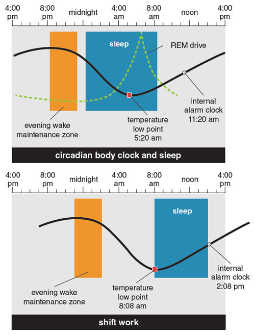
Adapted by Barbara Aulicino from FALPA.
In the United States, NASA established an international collaboration in the 1980s aimed at determining what factors contributed to fatigue, what the consequences were, and how the impact of these consequences might be mitigated. One such collaboration between NASA and the Federal Aviation Administration (FAA) relied heavily on the continuous collection of brain activity and eye-movement data, as well as subjective measurements (for instance, questionnaires) to determine the physiological alertness of pilots. This research provided valuable information about the effects on performance of work duration, time of day, and travel across time zones. One finding of particular interest was that a 40-minute rest period provided to pilots during long-haul flights significantly improved their alertness. Subsequent research has demonstrated that fatigue-related performance impairments fluctuate across the daily cycle of the circadian biological clock, so the risk of fatigue is greater at night and during the early hours of the morning. The risk of impairment also increases with the length of time spent awake, work duration, and work intensity, as evidenced across numerous laboratory and field studies. Although the research of the past few decades is now being used to develop formal guidelines for fatigue management, this wasn’t always the case.
Historically, fatigue has been addressed through a regulatory framework that specifies minimum rest periods and prescribes limits on work duration. These regulations originated during the Industrial Revolution, when the commonality of 10- to 16-hour working days under harsh conditions prompted social reformers, such as Robert Owens, to call for change. Owens is credited with coining the slogan, “Eight hours labor, eight hours recreation, and eight hours rest,” which reflected his belief that workers should be afforded a more equal distribution of life experiences over 24 hours. This concept eventually led to the establishment of regulations that stipulated how long employees could be asked to work.
However, in the early 1970s, opposition toward such policies began to grow. Albert Robens, an English politician and industrialist, criticized the regulations then in effect, faulting them for their excessive focus on the physical dimensions of work while giving little consideration to safety in the workplace. He encouraged the development of self-regulating systems for safety instead of regulatory approaches, which were deemed too complex to implement and sometimes ineffective at mitigating risk.
Consequently, in 1974 the United Kingdom’s Health and Safety at Work Act paved the way for a “performance-based” approach that set targets for safety without dictating how these targets would be achieved—an approach that was followed by other countries in the ensuing years. Inherent to this approach is the assumption that organizations are better able to understand and manage the risks associated with their specific activities than are regulatory agencies. Unlike previous regulations that placed responsibility for worker health and safety solely on the employer, the Health and Safety Act embodies a more uniform distribution of responsibilities between both parties. The employer must ensure the health and safety of workers by all means available; likewise, the employee must report for work duty in an acceptable state and must demonstrate safe behavior.
The most recent product of all these efforts has been the international adoption of fatigue risk management systems (FRMS) as an alternative to prescriptive limits on work duration. The FRMS, which both authors of this article have researched extensively, involves a continuous process of monitoring and managing the risk of fatigue and, according to its advocates, can either complement regulatory work–hour limitations or act as a substitute for them. In France, for example, the civil aviation authority allows an airline to grant rest periods to pilots that fall below regulatory limits if the airline also implements an FRMS. The airline must demonstrate that fatigue risk is managed at all levels, and it must prove explicitly that the reduced rest does not compromise safety as compared to a standard rest period—a requirement calling for specific provisions, such as proximity of the hotel to the airport, to reduce the flight crews’ travel time.
Other international air carriers have also applied FRMS principles. An extreme and necessary example is Qantas Airways, which currently operates one of the longest nonstop flights in the world: The journey from Sydney, Australia, to Dallas, Texas, covers some 8,500 miles and takes approximately 15.5 hours to complete. Such ultra-long haul flying exceeds regulatory limits and hence requires careful balancing of the work periods among the 15-plus flight attendants and pilots onboard to minimize the impact of fatigue.
Although the techniques described above are commendable efforts to mitigate fatigue, their implementation through regulatory rather than voluntary means is opposed by businesses for a number of reasons. Most important, the regulations start from the premise that the relationship between fatigue and safety is linear; that is, the more fatigued a person is, the higher the safety risk. This direct relationship may hold for human performance on fairly straightforward tasks such as driving (for example, falling asleep at the wheel increases the risk of crashing the vehicle), but such linearity is much more difficult to demonstrate in types of labor in which workers manage complex sociotechnical systems. Industries such as transportation and medicine, for instance, build in multiple layers of defenses with the explicit aim of reducing the likelihood of an accident attributable to a single cause like fatigue.
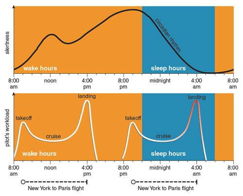
Illustration by Barbara Aulicino.
To take aviation again as an example, David Dawson and others have observed that the employees themselves rely on advanced technologies, checklists, resource management strategies, and defined operating procedures as protective mechanisms against the detrimental effects of fatigue. This observation may help explain seemingly counterintutive findings, such as that within the context of regional flights, Cabon and his collaborators have found that pilots provided with shorter rest opportunities between shifts (a minimum of 7 hours, 30 minutes instead of the standard rest of 13 hours) commit fewer errors than their more well-rested counterparts.
However, protective mechanisms can be a double-edged sword: At the same time that they reduce risk, they may convey an unrealistic sense of absolute safety. Although notions of what is safe vary greatly from one person to the next, passengers generally think of safety as a dichotomous state: Either an aircraft they are traveling on will experience a serious safety event or it will not. According to Arnold Barnett, a professor of statistics at the Massachusetts Institute of Technology, flying today has become so reliable that a passenger could fly every day for an average of 123,000 years before being in a fatal crash; understandably, therefore, we tend to think of it as safe. Mustering the political will to enact legislation for events that are so remote is a challenge at the conceptual level, even before practical considerations are taken into account.
As for the practical considerations, these are particularly weighty in the airline industry, because its structural constraints—high fixed costs and systemic overcapacity—act together to keep profit margins small. Estimates from the International Air Transportation Association (IATA), an airline trade group, put the industry-wide profit margin for 2014 at a mere 2.6 percent of revenue. To be sure, the amount in dollars is a staggering sum—on total revenues of $757 billion, the profit comes to $19.7 billion—but as pointed out by the director general of IATA, Tony Tyler, it is parceled out among hundreds of companies. The result is a profit of just $5.94 per passenger.
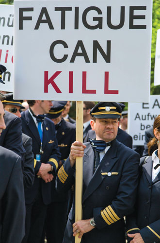
Carsten Koall/Getty Images
Such narrow profit margins, coupled with volatile fuel prices (which today account for up to 40 percent of operating expenses as compared with only 15 percent a few decades ago), mean that airlines are continuously looking for ways to cut costs. According to a report in the New York Times, Delta Airlines saved $250,000 in one year by shaving an ounce from each of the steaks it served on board, whereas American Airlines is said to have saved $40,000 a year by removing a single olive from every salad it served to passengers.
American Airlines is said to have saved $40,000 a year by removing a single olive from every salad it served to passengers.
Viewed strictly in terms of the bottom line, laws aimed at managing fatigue impede cost-cutting efforts by adding an extra layer of operating expenses to balance sheets that are already in the red. An example often cited on this point is a rule recently set by the FAA to minimize pilot fatigue by placing limits on night flying and the number of permissible daily takeoffs and landings. (The rule was prompted by the 2009 crash of Colgan Air Flight 3407 near Buffalo, New York, which killed all 49 passengers and was attributed, in part, to fatigue.)
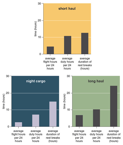
Adapted by Barbara Aulicino from FALPA.
The new rule requires that pilots get at least 10 hours of rest between shifts, including eight hours of uninterrupted sleep opportunity; recuperative periods of at least 30 consecutive hours each week; and work shifts that do not last more than nine hours. The FAA itself calculates these regulations will cost commercial airlines $306 million to implement, and at least one US airline has already attributed increased delays to its inability to schedule additional flights because pilots are “maxed out” under this new legislation.
Cargo carriers have successfully lobbied for exclusion from the rule altogether because the estimated implementation cost jumped to $550 million, a figure far above the $33 million in projected benefits associated with averting an accident. This exclusion appalled many—particularly in light of an estimate from the Air Line Pilots Association that the accident rate for cargo carriers is four to eight times higher than for passenger airlines. Robert Travis, president of the Independent Pilot’s Association, declared: “We do not believe that it was Congress’s intention to address the important issue of [pilot] fatigue only if the price is right.” The price is, however, an obstacle that has proved difficult to dislodge.
Opinion polls overwhelmingly show that customers are concerned about the impact of fatigue on air passengers’ safety and want to see stringent fatigue-management laws enacted. Yet these concerns are not borne out by their actions. The rapid rise of low-cost airlines in aviation is a testament to this inconsistency: Because the workforce represents an airline’s second-highest operating expense (the highest being fuel), a large portion of cost savings comes from maximizing the productivity of newly hired, low-pay workers. Many airlines now require flight attendants, for instance, to carry out additional tasks such as checking passenger tickets at the gate and cleaning aircraft cabins between flights. In some cases employees also work longer shifts, because low-cost airlines maximize the daily flying time of their aircraft by scheduling the first departure early in the morning and the last arrival late at night.
Clearly, customer concerns over fatigue are tempered by the prospect of flying from London to Frankfurt for $23.99.
Nor are pilots exempt from such working conditions: In 2006, a British television station used secret film to substantiate allegations that the low-cost airline Ryanair forced its pilots to work excessively fatiguing schedules by flying multiple consecutive flights a day through congested airspace with few opportunities for rest. How did customers respond? By helping Ryanair grow from a small, regional carrier to Europe’s largest airline, and a very profitable one, at a time when some of its competitors have been facing bankruptcy. According to IATA, in 2012 alone, Ryanair carried 30 million more international passengers than any other airline worldwide. The secret to Ryanair’s success is simple: low fares. Clearly, customer concerns over fatigue are tempered by the prospect of flying from London to Frankfurt for $23.99.
For all the challenges that safety advocates face in enacting fatigue legislation, the need to do so will become even more pressing in the future as the global labor force undergoes dramatic changes. These shifts can best be understood within the context of population aging, a megatrend that will fundamentally reshape societies for decades to come. The forces behind it are clear enough: People are having fewer children and living longer. Longevity may be seen as a human success story—the triumph of public health, medical advancements, and economic development over diseases and injuries that had limited human life expectancy for millennia. Yet longevity in the presence of declining fertility is altering population structures in ways that will have profound economic consequences. This is because population aging reduces the relative size of the labor force as fewer new workers are available to replace those who retire.
According to a Boston consulting group report, 2010 saw 0.3 people retiring for each person entering the workforce; by 2050, that number will be 0.7. For advanced industrial countries, the figures are even worse: from 0.8 retirees per new worker in 2010, the ratio is expected to climb to one retiree per worker in 2050. The immediate impact of fewer workers is an inability of companies to meet service demand, which can lead to the stagnation of economic growth seen in some sectors across China and Indonesia, where skilled labor shortages are commonplace.
Fully aware of the economic fallout associated with lost productivity, employers are responding to these shortages by implementing policies that require higher levels of effort from the existing workforce. In aviation, for example, steadily increasing flight activity at the Vienna International Airport was recently disrupted when a dispute broke out between air traffic controllers and their management. The employees demanded significant reductions in mandatory overtime hours; the management refused, on the grounds that additional hours were a reasonable requirement to avoid financial damage to the company and to minimize service disruption to the flying public. In medicine, a 2010 survey by the Royal College of Nursing in Scotland found that just one in 10 nurses felt staffing levels were adequate at their workplace. An overwhelming majority of nurses, 98 percent, reported working longer than their contracted hours, with more than a quarter (27 percent) reporting this was done during consecutive shifts. The findings led to accusations that nurses were “propping up” the British National Health Service by repeatedly working more hours than contracted and providing last-minute shift cover to make up for staffing shortages.
Although such managerial policies may be understandable as a short-term means of coping with labor shortages, they raise serious concerns about worker fatigue. Equally important, they raise the possibility of questions about the quality of services those fatigued workers are capable of providing.
Perhaps technology can provide solutions as scientific advances facilitate the creation of a brave new world—one in which increasing service demand can be effortlessly satisfied with fewer workers, simply by an increasing reliance on automation. Such advances, coupled with a dramatic fall in the price of technology over the past half-century, make this prospect possible. It may not, however, be entirely plausible.
Technological advances have led to the production of machines that can replace humans on some tasks—those that follow formal rules and procedures—but such machines are less appropriate for work that calls for creative problem-solving. The tasks carried out by doctors, for example, are notoriously difficult to automate, because they do not follow a defined pattern. Rather, the blend of complex biology and many overlays of social, psychological, and economic issues make the practice of medicine a complicated, nuanced affair. Physicians and other healthcare workers must creatively adapt to changing situational demands, a process that engineers have been unable to replicate thus far by means of technology.
DA Photo/Alamy
Moreover, the safety-critical nature of some industries highlights the need for human involvement regardless of the role of technology. For example, although commercial airliners can now land in zero-visibility conditions with no human input, a pilot is needed to ensure that the rules followed by technology are appropriate in the circumstances. More important is the overwhelming concern that should technology fail, a pilot will still be needed to recover from what could be a life-threatening situation.
Hence, occupations within specific industries such as transportation, medicine, and industry still face the challenge of addressing worker fatigue, while catering to an increasing demand for service with a shrinking workforce. Psychologists, physiologists, and economists will need to collaborate to address fundamental questions such as: What are the trade-offs of cost, safety, and efficiency at varying levels of shift duration and intensity for workers? What types of technology are most appropriate to supplement workforce capabilities? Perhaps most important, what are the optimal conditions under which humans and technology can work together to ensure seamless operations? As these industries continue to gain social influence and economic power, the need to address this challenge through legislation that balances the requirements of business, workers, and the general public will become even more pressing. Whether this challenge can be met is a matter that should concern us all. With all due recognition of the capabilities that new technology offers, we do well to remember that in unexpected circumstances, when technology is most likely to behave unreliably, humans will still be called upon to act as a backup, fulfilling our role as ultimate guardians of complex systems.
Click "American Scientist" to access home page

American Scientist Comments and Discussion
To discuss our articles or comment on them, please share them and tag American Scientist on social media platforms. Here are links to our profiles on Twitter, Facebook, and LinkedIn.
If we re-share your post, we will moderate comments/discussion following our comments policy.