American Scientist

Why are some computational problems so hard and others easy? This may sound like a childish, whining question, to be dismissed with a shrug or a wisecrack, but if you dress it up in the fancy jargon of computational complexity theory, it becomes quite a serious and grownup question: Is P equal to NP? An answer—accompanied by a proof—will get you a million bucks from the Clay Mathematics Institute.

I'll return in a moment to P and NP, but first an example, which offers a glimpse of the mystery lurking beneath the surface of hard and easy problems. Consider a mathematical graph, a collection of vertices (represented by dots) and edges (lines that connect the dots). Here's a nicely symmetrical example:

Is it possible to construct a path that traverses each edge exactly once and returns to the starting point? For any graph with a finite number of edges, we could answer such a question by brute force: Simply list all possible paths and check to see whether any of them meet the stated conditions. But there's a better way. In 1736 Leonhard Euler proved that the desired path (now called an Eulerian circuit) exists if and only if every vertex is the end point of an even number of edges. We can check whether a graph has this property without any laborious enumeration of pathways.

Now take the same graph and ask a slightly different question: Is there a circuit that passes through every vertex exactly once? This problem was posed in 1858 by William Rowan Hamilton, and the path is called a Hamiltonian circuit. Again we can get the answer by brute force. But in this case there is no trick like Euler's; no one knows any method that gives the correct answer for all graphs and does so substantially quicker than exhaustive search. Superficially, the two problems look almost identical, but Hamilton's version is far harder. Why? Is it because no shortcut solution exists, or have we not yet been clever enough to find one?

Most computer scientists and mathematicians believe that Hamilton's problem really is harder, and no shortcut algorithm will ever be found—but that's just a conjecture, supported by experience and intuition but not by proof. Contrarians argue that we've hardly begun to explore the space of all possible algorithms, and new problem-solving techniques could turn up at any time. Before 1736, the Eulerian-circuit problem also looked hard.

What prompts me to write on this theme is a new and wholly unexpected family of algorithms that provide efficient methods for several problems that previously had only brute-force solutions. The algorithms were invented by Leslie G. Valiant of Harvard University, with extensive further contributions by Jin-Yi Cai of the University of Wisconsin. Valiant named the methods "holographic algorithms," but he also refers to them as "accidental algorithms," emphasizing their capricious, rabbit-from-the-hat quality; they seem to pluck answers from a tangle of unlikely coincidences and cancellations. I am reminded of the famous Sidney Harris cartoon in which a long series of equations on a blackboard hinges on the notation "Then a miracle occurs."

The Coffee-Break Criterion

For most of us, the boundary between fast and slow computations is clearly marked: A computation is slow if it's not finished when you come back from a coffee break. Computer science formalizes this definition in terms of polynomial-time and exponential-time algorithms.

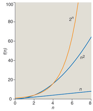
Suppose you are running a computer program whose input is a list of n numbers. The program might be sorting the numbers, or finding their greatest common divisor, or generating permutations of them. No matter what the task, the running time of the program will likely depend in some way on n, the length of the list (or, more precisely, on the total number of bits needed to represent the numbers). Perhaps the time needed to process n items grows as n². Thus as n increases from 10 to 20 to 30, the running time rises from 100 to 400 to 900. Now consider a program whose running time is equal to 2ⁿ. In this case, as the size of the input grows from 10 to 20 to 30, the running time leaps from a thousand to a million to a billion. You're going to be drinking a lot of coffee.

The function n² is an example of a polynomial; 2ⁿ denotes an exponential. The distinction between these categories of functions marks the great divide of computational complexity theory. Roughly speaking, polynomial algorithms are fast and efficient; exponential algorithms are too slow to bother with. To speak a little less roughly: When n becomes large enough, any polynomial-time program is faster than any exponential-time program.

So much for the classification of algorithms. What about classifying the problems that the algorithms are supposed to solve? For any given problem, there might be many different algorithms, some faster than others. The custom is to rate a problem according to the worst-case performance of the best algorithm. The class known as P includes all problems that have at least one polynomial-time algorithm. The algorithm has to give the right answer and has to run in polynomial time on every instance of the problem.

Classifying problems for which we don't know a polynomial-time algorithm is where it gets tricky. In the first place, there are some problems that require exponential running time for reasons that aren't very interesting. Think about a program to generate all subsets of a set of n items; the computation is easy, but because there are 2ⁿ subsets, just writing down the answer will take an exponential amount of time. To avoid such issues, complexity theory focuses on problems with short answers. Decision problems ask a yes-or-no question ("Does the graph have a Hamiltonian circuit?"). There are also counting problems ("How many Hamiltonian circuits does the graph have?"). Problems of these kinds might conceivably have a polynomial-time solution, and we know that some of them do. The big question is whether all of them do. If not, what distinguishes the easy problems from the hard ones?

Conscientious Cheating

The letters NP might well be translated "notorious problems," but the abbreviation actually stands for "nondeterministic polynomial." The term refers to a hypothetical computing machine that can solve problems through systematic guesswork. For the problems in NP, you may or may not be able to compute an answer in polynomial time, but if you happen to guess the answer, or if someone whispers it in your ear, then you can quickly verify its correctness. NP is the complexity class for conscientious cheaters—students who don't do their own homework but who at least check their cribbed answers before they turn them in.

Detecting a Hamiltonian circuit is one example of a problem in NP. Even though I don't know how to solve the problem efficiently for all graphs, if you show me a purported Hamiltonian circuit, I can readily check whether it passes through every vertex once:

(Note that this verification scheme works only when the answer to the decision problem is "yes." If you claim that a graph doesn't have a Hamiltonian circuit, the only way to prove it is to enumerate all possible paths.)

Within the class NP dwells the elite group of problems labeled NP-complete. They have an extraordinary property: If any one of these problems has a polynomial-time solution, then that method can be adapted to quickly solve all problems in NP (both the complete ones and the rest). In other words, such an algorithm would establish that P = NP. The two categories would merge.

The very concept of NP-completeness has a whiff of the miraculous about it. How can you possibly be sure that a solution to one problem will work for every other problem in NP as well? After all, you can't even know in advance what all those problems are. The answer is so curious and improbable that it's worth a brief digression.

The first proof of NP-completeness, published in 1971 by Stephen A. Cook of the University of Toronto, concerns a problem called satisfiability. You are given a formula in Boolean logic, constructed from a set of variables, each of which can take on the values true or false, and the logical connectives AND, OR and NOT. The decision problem asks: Is there a way of assigning true and false values to the variables that makes the entire formula true? With n variables there are 2ⁿ possible assignments, so the brute-force approach is exponential and unappealing. But a lucky guess is easily verified, so the problem qualifies as a member of NP.

Cook's proof of NP-completeness is beautiful in its conception and a shambling Rube Goldberg contraption in its details. The key insight is that Boolean formulas can describe the circuits and operations of a computer. Cook showed how to write an intricate formula that encodes the entire operation of a computer executing a program to guess a solution and check its correctness. If and only if the Boolean formula has a satisfying assignment, the simulated computer program succeeds. Thus if you could determine in polynomial time whether or not any Boolean formula is satisfiable, you could also solve the encoded decision problem. The proof doesn't depend on the details of that problem, only on the fact that it has a polynomial-time checking procedure.

Thousands of problems are now known to be NP-complete. They form a vast fabric of interdependent computations. Either all of them are hard, or everything in NP is easy.

The Match Game

To understand the new holographic algorithms, we need one more ingredient from graph theory: the idea of a perfect matching.

Consider the double-feature festival. You want to show movies in pairs, with the proviso that any two films scheduled together should have a performer in common; also, no film can be screened more than once. These constraints lead to a graph where the vertices are film titles, and two titles are connected by an edge if the films share an actor. The task is to identify a set of edges linking each vertex to exactly one other vertex. The brute-force method of trying all possible matchings is exponential, but if you are given a candidate solution, you can efficiently verify its correctness:

Thus the perfect-matching problem lies in NP.

In the 1960s Jack Edmonds, now of the University of Waterloo, devised an efficient algorithm that finds a perfect matching if there is one. The Edmonds algorithm works in polynomial time, which means the decision problem for perfect matching is in P. (Indeed, Edmonds's 1965 paper includes the first published discussion of the distinction between polynomial and exponential algorithms.)

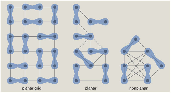
Another success story among matching methods applies only to planar graphs—those that can be drawn without crossed edges. On a planar graph you can efficiently solve not only the decision problem for perfect matching but also the counting problem—that is, you can learn how many different subsets of edges yield a perfect matching. In general, counting problems seem more difficult than decision problems, since the solution conveys more information. The main complexity class for counting problems is called #P (pronounced "sharp P"); it includes NP as a subset, so #P problems must be at least as hard as NP.

The problem of counting planar perfect matchings has its roots in physics and chemistry, where the original question was: If diatomic molecules are adsorbed on a surface, forming a single layer, how many ways can they be arranged? Another version asks how many ways dominos (2-by-1 rectangles) can be placed on a chessboard without gaps or overlaps. The answers exhibit clear signs of exponential growth; when you arrange dominos on square boards of size 2, 4, 6 and 8, the number of distinct tilings is 2, 36, 6,728 and 12,988,816. Given this rapid proliferation, it seems quite remarkable that a polynomial-time algorithm can count the configurations. The ingenious method was developed in the early 1960s by Pieter W. Kasteleyn and, independently, Michael E. Fisher and H. N. V. Temperley. It has come to be known as the FKT algorithm.

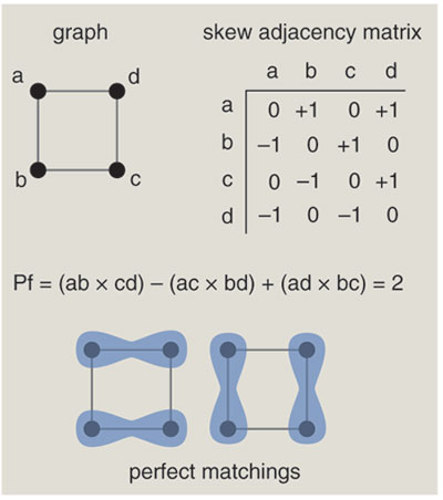
The mathematics behind the FKT algorithm takes some explaining. In outline, the idea is to encode the structure of an n-vertex graph in an n-by-n matrix; then the number of perfect matchings is given by an easily computed property of the matrix. The illustration (above right) shows how the graph is represented in matrix form.

The computation performed on the matrix is essentially the evaluation of a determinant. By definition, a determinant is a sum of n! terms, where each term is a product of n elements chosen from the matrix. The symbol n! denotes the factorial of n, or in other words n×(n–1)×...×3×2×1. The trouble is, n! is not a polynomial function of n; it qualifies as an exponential. Thus, under the rules of complexity theory, the whole scheme is really no better than the brute-force enumeration of all perfect matchings. But this is where the rabbit comes out of the hat. There are alternative algorithms for computing determinants that do achieve polynomial performance; the best-known example is the technique called Gaussian elimination. With these methods, all but a polynomial number of terms in that giant summation magically cancel out. We never have to compute them, or even look at them.

(The answer sought in the perfect-matching problem is actually not the determinant but a related quantity called the Pfaffian. However, the Pfaffian is equal to the square root of the determinant, and so the computational procedure is essentially the same.)

The existence of a shortcut for evaluating determinants and Pfaffians is like a loophole in the tax code—a windfall for those who can take advantage of it, but you can only get away with such special privileges if you meet very stringent conditions.

Closely related to the determinant is another quantity associated with matrices called the permanent. It's another sum of n! products, but even simpler. For the determinant, a complicated rule assigns positive and negative signs to the various terms of the summation. For the permanent, there's no need to bother keeping track of the signs; they're all positive. But the alternation of signs is necessary for the cancellations that allow fast computation of determinants. As a result, the polynomial loophole doesn't work for permanents. In 1979 Valiant showed that the calculation of permanents is #P-complete. (It was in this work that the class #P was first defined.)

At a higher level, too, the conspiracy of circumstances that allows perfect matchings to be counted in polynomial time seems rather delicate and sensitive to details. The algorithm works only for planar graphs; attempts to extend it to larger families of graphs have failed. Even for planar graphs, it works only for perfect matchings; counting the total number of matchings is a #P-complete task.

Algorithmic Holography

The engine that drives the FKT algorithm is the linear-algebra shortcut for evaluating determinants (or Pfaffians) in polynomial time. This prime mover is harnessed to solve a counting problem in another area of mathematics, namely graph theory. Such translations, or "reductions," from one problem to another are standard fare in complexity theory. Holographic algorithms also rely on reductions, and indeed they ultimately translate problems into the language of determinants. But the nature of the reductions is novel.

A typical non-holographic reduction is a one-to-one mapping between problems in two domains. If you can reduce problem A to problem B, and then find a solution to an instance of B, you know that the corresponding instance of A also has a solution. Devising transformations that set up this one-to-one linkage between problems is a demanding art form. Holographic reductions exploit a broader class of transformations that don't necessarily link individual problem instances, but the reductions do preserve the number of solutions or the sum of the solutions. For certain counting problems, that's enough.

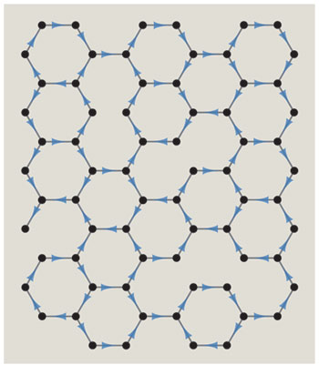
A problem with the cryptic name #PL-3-NAE-ICE supplies an example of the holographic process. The problem concerns a planar graph of maximum degree three; that is to say, no vertex has more than three edges. Each edge is to be assigned a direction, subject to the constraint that no vertex of degree two or three can have all of its edges directed either inward or outward. Graphs of this general kind have been studied as models of the structure of ice; the vertices represent molecules and the directed edges are chemical bonds. The decision version of the problem asks whether the edges can be assigned directions so that the not-all-equal constraint is obeyed everywhere. Here we are interested in the counting version, which asks how many ways the constraints can be satisfied.

The strategy is to build a new planar graph called a matchgrid, which encodes both the structure of the ice graph and the not-all-equal constraints that have to be satisfied at each vertex. Then we calculate a weighted sum of the perfect matchings in the matchgrid, using the efficient FKT algorithm. Although there may be no one-to-one mapping between individual matchings in the matchgrid and valid assignments of bond directions in the ice graph, the weighted sum of the perfect matchings is equal to the number of valid assignments.

The matchgrid is constructed from components called matchgates, which are planar graph fragments that act much like the logic gates of Boolean circuits. To understand how this computer built of graphs works, it helps to consider first an idealized and simplified version, in which we can manufacture matchgates to meet any specifications we please.

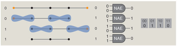
Given such an unlimited stock of gates, we can assemble a model of PL-3-NAE-ICE as follows. A degree-three vertex in the ice graph is represented by a "recognizer" matchgate with three inputs. The recognizer has a "signature" that implements the not-all-equal function: the gate is designed so that its contribution to the sum of the perfect matchings is 0 if the three inputs are 000 or 111, but the contribution is 1 for any of the other six possible input patterns (001, 010, 011, 100, 101, 110).

Each edge of the ice graph is represented in the matchgrid by a "generator" matchgate that has two outputs, corresponding to the two ends of the edge. To capture the idea that an edge has a direction—pointing toward one end and away from the other—the generator contributes 1 to the weighted sum when the outputs are either 01 or 10, but the contribution is 0 for outputs 00 and 11.

In this scheme, the concept of perfect matching becomes a computational mechanism. If a graph fragment, packaged up as a matchgate, allows a perfect matching, then the gate outputs a logical 1, or true. If no perfect matching is possible, the output is 0, or false. This is a novel and interesting way to build a computer, but there's a catch. Many of the needed matchgates cannot be implemented in the direct manner described above. In particular, the three-input not-all-equal gate cannot be implemented. The reason is easy to demonstrate. Perfect matching is all about parity; a graph cannot possibly have a perfect matching unless the number of vertices is even. The three-input not-all-equal gate is required to respond in the same way to the inputs 000 and 111. But these patterns have opposite parity; one is even and the other is odd.

The remedy for this impediment is yet more linear algebra. Although no simple matchgate can directly implement the three-input not-all-equal function, the desired behavior can be generated as a linear superposition of other functions. Finding an appropriate set of equations to create such superpositions is the most essential and also the most difficult aspect of applying the holographic method. It has mostly been a hit-or-miss proposition, requiring both inspiration and expert use of computer-algebra systems. Cai and Pinyan Lu of Tsinghua University have recently made progress on systematizing the search process.

So far about a dozen counting problems have been solved by the holographic method, none of them having any immediate practical use or consequences for the further development of complexity theory. Indeed, they are an odd lot—apart from the ice problem they are mostly specialized and restricted versions of satisfiability and matching. One particularly curious result gives a fast algorithm for counting a certain set of solutions modulo 7, but counting the same set modulo 2 is at least as hard as NP-complete.

Why are the methods called holographic algorithms? Valiant explains that their computational power comes from the mutual cancellation of many contributions to a sum, as in the optical interference pattern that creates a hologram. This sounds vaguely like the superposition principle in quantum computing, and that is not entirely a coincidence. Valiant's first publication on the topic, in 2002, was titled "Quantum circuits that can be simulated classically in polynomial time."

P or NP, That Is the Question

Do holographic algorithms reveal anything we didn't already know about the P = NP question? Lest there be any misunderstanding, one point bears emphasizing: Although some of the problems solved by holographic methods were not previously known to be in P, none of them were NP-complete or #P-complete. Thus, so far, the barrier between P and NP remains intact.

Suggesting that P might be equal to NP is deeply unfashionable. A few years ago William Gasarch of the University of Maryland took a poll on the question. Of 100 respondents, only nine stood on the side of P = NP, and Gasarch reported that some of them took the position "just to be contrary." The idea that all NP problems have easy solutions seems too good to be true, an exercise in wishful thinking; it would be miraculous if we lived in a universe where computing is so effortless. But the miracle argument cuts both ways: For NP to remain aloof from P, we have to believe that not even one out of all those thousands of NP-complete problems has an efficient solution.

Valiant suggests a comparison with the Goldbach conjecture, which holds that every even number greater than 2 is the sum of two primes. Nearly everyone believes it to be true, but in the absence of a proof, we don't know why it should be true. We can't rule out the possibility that exceptions exist but are so rare we haven't stumbled on one yet. Likewise with the P and NP question: A polynomial algorithm for just one NP-complete problem would forever alter the landscape.

The work on holographic algorithms doesn't have to be seen as some sort of wildcat drilling expedition, hoping to strike a P = NP gusher. It would be worthwhile just to have a finer survey of the boundaries between complexity classes, showing more clearly what can and can't be accomplished with polynomial resources. Valiant writes that "any proof of P ? NP will need to explain, and not only to imply, the unsolvability of our polynomial systems."

Finally, there's the challenge of understanding the algorithms themselves at a deeper level. To call them "accidental"—or "exotic," or "freak," which are other terms that turn up in the literature—suggests that they are sports of nature, like weird creatures found under a rock and put on exhibit. But one could also argue, on the contrary, that these algorithms are not at all accidental; they are highly engineered constructions. The elaborate systems of polynomials needed to create sets of matchgates are not something found in the primordial ooze of mathematics. Someone had to invent them.

© Brian Hayes