What Everyone Should Know about Statistical Correlation
By Vladica Velickovic
A common analytical error hinders biomedical research and misleads the public.
A common analytical error hinders biomedical research and misleads the public.

DOI: 10.1511/2015.112.26
In 2012, the New England Journal of Medicine published a paper claiming that chocolate consumption could enhance cognitive function. The basis for this conclusion was that the number of Nobel Prize laureates in each country was strongly correlated with the per capita consumption of chocolate in that country. When I read this paper I was surprised that it made it through peer review, because it was clear to me that the authors had committed two common mistakes I see in the biomedical literature when researchers perform a correlation analysis.

Correlation describes the strength of the linear relationship between two observed phenomena (to keep matters simple, I focus on the most commonly used linear relationship, or Pearson’s correlation, here). For example, the increase in the value of one variable, such as chocolate consumption, may be followed by the increase in the value of the other one, such as Nobel laureates. Or the correlation can be negative: The increase in the value of one variable may be followed by the decrease in the value of the other. Because it is possible to correlate two variables whose values cannot be expressed in the same units—for example, per capita income and cholera incidence—their relationship is measured by calculating a unitless number, the correlation coefficient. The correlation coefficient ranges in value from –1 to +1. The closer the magnitude is to 1, the stronger the relationship.
The stark simplicity of a correlation coefficient hides the considerable complexity in interpreting its meaning. One error in the New England Journal of Medicine paper is that the authors fell into an ecological fallacy, when a conclusion about individuals is reached based on group-level data. In this case, the authors calculated the correlation coefficient at the aggregate level (the country), but then erroneously used that value to reach a conclusion about the individual level (eating chocolate enhances cognitive function). Accurate data at the individual level were completely unknown: No one had collected data on how much chocolate the Nobel laureates consumed, or even if they consumed any at all. I was not the only one to notice this error. Many other scientists wrote about this case of erroneous analysis. Chemist Ashutosh Jogalekar wrote a thorough critique on his Scientific American blog The Curious Wavefunction, and Beatrice A. Golomb of University of California, San Diego, even tested this hypothesis with a team of coauthors, pointing out that there is no link.
Regardless of the scientific community’s criticism of this paper, many news agencies reported on this article’s results. The paper was never retracted, and to date has been cited 23 times. Even when erroneous papers are retracted, news reports about them remain on the Internet and can continue to spread misinformation. If these faulty conclusions reflecting statistical misconceptions can appear even in the New England Journal of Medicine, I wondered, how often are they appearing in the biomedical literature generally?
The example of chocolate consumption and Nobel Prize winners brings me to another, even more common misinterpretation of correlation analysis: the idea that correlation implies causality. Calculating a correlation coefficient does not explain the nature of a quantitative agreement; it only assesses the intensity of that agreement. The two factors may show a relationship not because they are influenced by each other but because they are both influenced by the same hidden factor—in this case, perhaps a country’s affluence affects access to chocolate and the availability of higher education. Correlation can certainly point to a possible existence of causality, but it is not sufficient to prove it.
An eminent statistician, George E. P. Box, wrote in his book Empirical Model Building and Response Surfaces: “Essentially, all [statistical] models are wrong, but some are useful.” All statistical models are a description of a real-world phenomenon using mathematical concepts; as such, they are just a simplification of reality. If statistical analyses are carefully designed, in accordance with current good practice guidelines and a thorough understanding of the limitations of the methods used, they can be very useful. But if models are not designed in accordance with the previous two principles, they can be not only inaccurate and completely useless but also potentially dangerous—misleading medical practitioners and public.
I often use and design mathematical models to gain insight into public health problems, especially in health technology assessment. For this purpose I use data from already published studies. Uncritical use of published data for designing these models would lead to inaccurate, completely useless—or worse, unsafe—conclusions about public health.
In well-designed experiments, correlation can confirm the existence of causality. Before causal inferences can be derived from nonexperimental data, however, careful statistical modeling must be used. For example, a randomized controlled trial published by epidemiologist Stephen Hulley of University of California, San Francisco, and colleagues determined that hormone replacement therapy caused increased risk of coronary heart disease, even though previously published nonexperimental studies concluded that the therapy lowered its risk. The well-designed experiment showed that the lower-than-average incidence of coronary heart disease in the nonexperimental studies was caused by the benefits associated with a higher average socioeconomic status of those using the hormone treatment, not by the therapy itself. Re-analyses of nonexperimental studies, including the effect of socioeconomic status on outcome, showed the same findings as the randomized controlled trial. But the damage was done: The US Food and Drug Administration Advisory Committee had already approved a label change for hormone replacement therapy that permitted prevention of heart disease to be included as an indication, almost a decade before the experiment mentioned above.
Even though scientists are well aware of the mantra “correlation does not equal causation,” studies conflating correlation and causation are all too common in leading journals. A widely discussed 1999 article in Nature found a strong association between myopia and night-time ambient light exposure during sleep in children under two years of age. However, another study published a year later—also in Nature—refuted these findings and reported that the cause of child myopia is genetic, not environmental. This new study found a strong link between parental myopia and the development of child myopia, noting that myopic parents were also incidentally more likely to leave a light on in their children’s bedroom. In this example, authors came to a conclusion based on a spurious correlation, without checking for other likely explanations. But as shown in the figure below, completely, laughably unrelated phenomena can be correlated.
Along with the mistaken idea that correlation implies causation, I also see examples of a third, opposite type of correlation error: the belief that a correlation of zero implies independence. If two variables are independent of one another—for example, the number of calories I ate for breakfast over the past month and the temperature of the Moon’s surface over the same period—then I would expect the linear correlation coefficient between them to be zero. The reverse is not always the case, however. A linear correlation coefficient of zero does not necessarily mean that the two variables are independent.
Although this principle can be applied in many cases, there are still nonmonotonic relationships (think of a line graph that goes up and down) in which the value of the correlation coefficient equaling zero will not imply independence. To better envision this abstract concept, imagine flipping a fair coin to determine the amount of a bet, using the following rule: When heads is flipped first and then tails, you lose $10; if tails comes up first and then heads, you win $20. If we define X as the amount of the bet and Y as the net winning, X and Y may have zero correlation, but they will not be independent—indeed, if you know the value of X, then you know the value of Y. Nevertheless, the relationship between the two variables may be nonlinear, and thus not detected by a linear correlation test.
Ideally, a scientist would plot the data first to make sure it is monotonic (steadily increasing or decreasing), but judging from the examples I see in the biomedical literature, some people are cutting corners. A U-shaped relationship between two variables may have a linear correlation coefficient of zero, but in that case it does not imply that the variables are independent.
In 1973, Frank Anscombe, a statistician from England, developed idealized data sets to graphically demonstrate this misconception. Called Anscombe’s quartet, this representation shows four data sets that have very similar statistical properties, each with a correlation coefficient of 0.816. On first blush, the variables in each case appear to be strongly correlated. However, it is enough just to observe the plots of these four data sets to realize that such a conclusion is wrong (see figure below). Only the first graph clearly shows a linear relationship where the interpretation of a very strong correlation would be appropriate. The second and the fourth graphs show that the relationship between the two variables is not linear, and so the correlation coefficient of 0.816 would not be relevant. The third graph depicts an almost perfect relationship in which the linear correlation coefficient value should be almost 1, but a single outlier decreases the linear correlation coefficient value to 0.816.
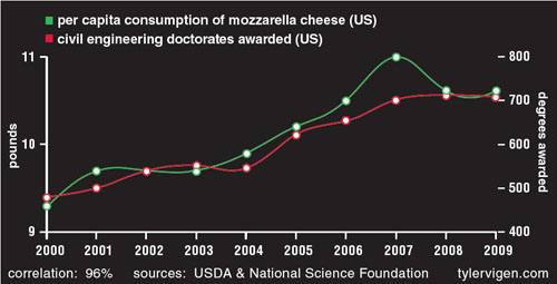
Illustration by Tom Dunne.
Such misconceptions can have major impacts on human health and policy. When testing the safety of a new substance, toxicologists often assume that high-dose tests will reveal low-dose effects more quickly and with less ambiguity than long-period, low-dose testing. But Anderson Andrade of the Charité University Medical School and his colleagues showed otherwise. They tested the effect of a plastic ingredient and endocrine disruptor called DEHP (di-(2-ethylhexyl)-phthalate) on rats at two widely different levels of exposure; in the experiment, the researchers monitored the activity of a key enzyme called aromatase, which induces masculinization in the brain. They showed that lower doses of DEHP suppress aromatase, but higher doses actually increase the enzyme’s activity.
In Andrade’s study, this dose-response curve follows a nonmonotonic pattern, and the usual high-dose tests would not predict these low-dose effects. In 2010, the US Consumer Product Safety Commission announced that products containing DEHP may be considered toxic and hazardous. Studies such as this one have led to the questioning of basic assumptions used to design toxicological tests of hormonally active compounds, and this example again confirms that sloppy analysis, or poor and superficial interpretation of data, certainly is not a benign phenomenon.
All three misinterpretations of correlation can be avoided. Epidemiologist and statistician Austin Bradford Hill suggested in 1965 certain criteria that must be met to justify concluding causal associations. Those criteria are still valid, but newer methods for drawing causal inference from observational data have also been developed. Others are still in development—for example, Judea Pearl and James Robins independently introduced a new framework for drawing causal inference from non-experimental studies. Robins figured out a statistical solution that can convert nonexperimental data into data like those resulting from a randomized controlled trial.
To avoid an ecological inference fallacy, Hill suggests that researchers who lack data at the individual level should perform careful multilevel modeling. This kind of fallacy is often made in epidemiological studies when researchers only have access to aggregate data. In his 1997 book A Solution to the Ecological Inference Problem, Gary King of Harvard University describes the statistical difficulties that lead to such errors. As King explains, data used for ecological inferences tend to have massive levels of heteroskedasticity, meaning that the variability within different parts of a data set fluctuates widely across the range of values.
Aggregate data are often easier to obtain than data on individuals and may offer valuable clues about individual behavior when analyzed correctly, but that requires individual-level data. Then, modeling at the individual level must be performed in an attempt to determine the connection between individual and aggregate levels. Only then is it possible to conclude whether the correlation at the aggregate level applies to the individual level. Ecologic data alone do not allow one to determine whether ecologic bias is likely to be present for this type of data set; the only solution is to supplement the ecologic data with individual-level data. This type of modeling usually involves mixed or multilevel statistical models, which allow for individuals to be nested into aggregates.
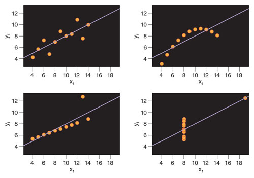
Illustration by Tom Dunne.
To avoid assuming two variables are independent because their correlation equals zero, the data must be plotted to make sure it is monotonic. If not, one or both variables can be transformed to make them so. In a transformation, all values of a variable are recalculated using the same equation, so that the relationship between the variables is maintained but their distribution is changed. Different types of transformations are used for different distributions; for example, the logarithmic transformation compresses the spacing between large values and stretches out the spacing between small values, which is appropriate when groups of values with larger means also have larger variance. Without access to the original data, it is impossible to know whether this error has been committed.
Correlation errors are as old as statistics itself, but as the number of published papers and new journals continues to increase, errors multiply as well. Although it is not realistic to expect all researchers to have an in-depth knowledge of statistical methods, they must continuously monitor and extend basic methodological knowledge. Ignorance or uncritical assessment of the adequacy and limitations of statistical methods used often are the source of errors in academic papers. Involvement of biostatisticians and mathematicians in a research team is no longer an advantage but a necessity. Some universities offer the option for researchers to check their analysis with their statistics department before sending the article to review with a publication. Although this solution could work for some researchers, it provides little incentive for the researcher to take this extra time.
Involvement of biostatisticians and mathematicians in a research team is no longer an advantage but a necessity.
The process of scientific research requires adequate knowledge of biostatistics, a constantly changing field. To that end, biostatisticians should be involved in the research from the very beginning, not after the measurement, observations, or experiments are completed. On the other hand, basic knowledge of biostatistics is essential in the critical appraisal of published scientific papers. A critical approach must exist regardless of the journal in which the paper is published. A more careful use of statistics in biology can also help set more rigorous standards for other fields.
To avoid these problems, scientists must clearly show that they understand the assumptions behind a statistical analysis and explain in their methods what they have done to make sure their data set meets those assumptions. A paper should not make it through review if these best practices are not followed. To make it possible for reviewers to test and replicate analyses, the following three principles must become mandatory for all authors intending to publish results: publishing data sets as supplementary information alongside articles, giving reviewers full access to the software code used for the analysis, and registering the study in a publicly available database online with clearly stated study objectives before the beginning of research, with mandatory submission of summary results to avoid publication bias toward positive results. These steps could speed up the process of detecting errors even when reviewers miss them, provide increased transparency to bolster confidence in science, and, most important, avoid damage to public health caused by unintentional errors.
Click "American Scientist" to access home page

American Scientist Comments and Discussion
To discuss our articles or comment on them, please share them and tag American Scientist on social media platforms. Here are links to our profiles on Twitter, Facebook, and LinkedIn.
If we re-share your post, we will moderate comments/discussion following our comments policy.